GNSS/IMU-Positioning Urban Challenges #2: Forests

Short intro and dataset
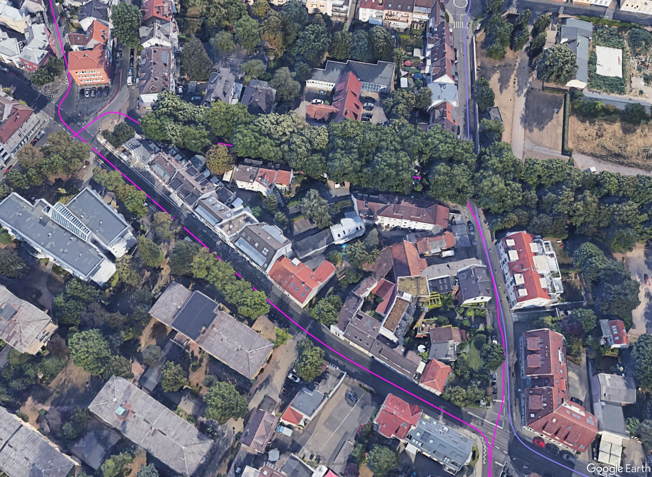
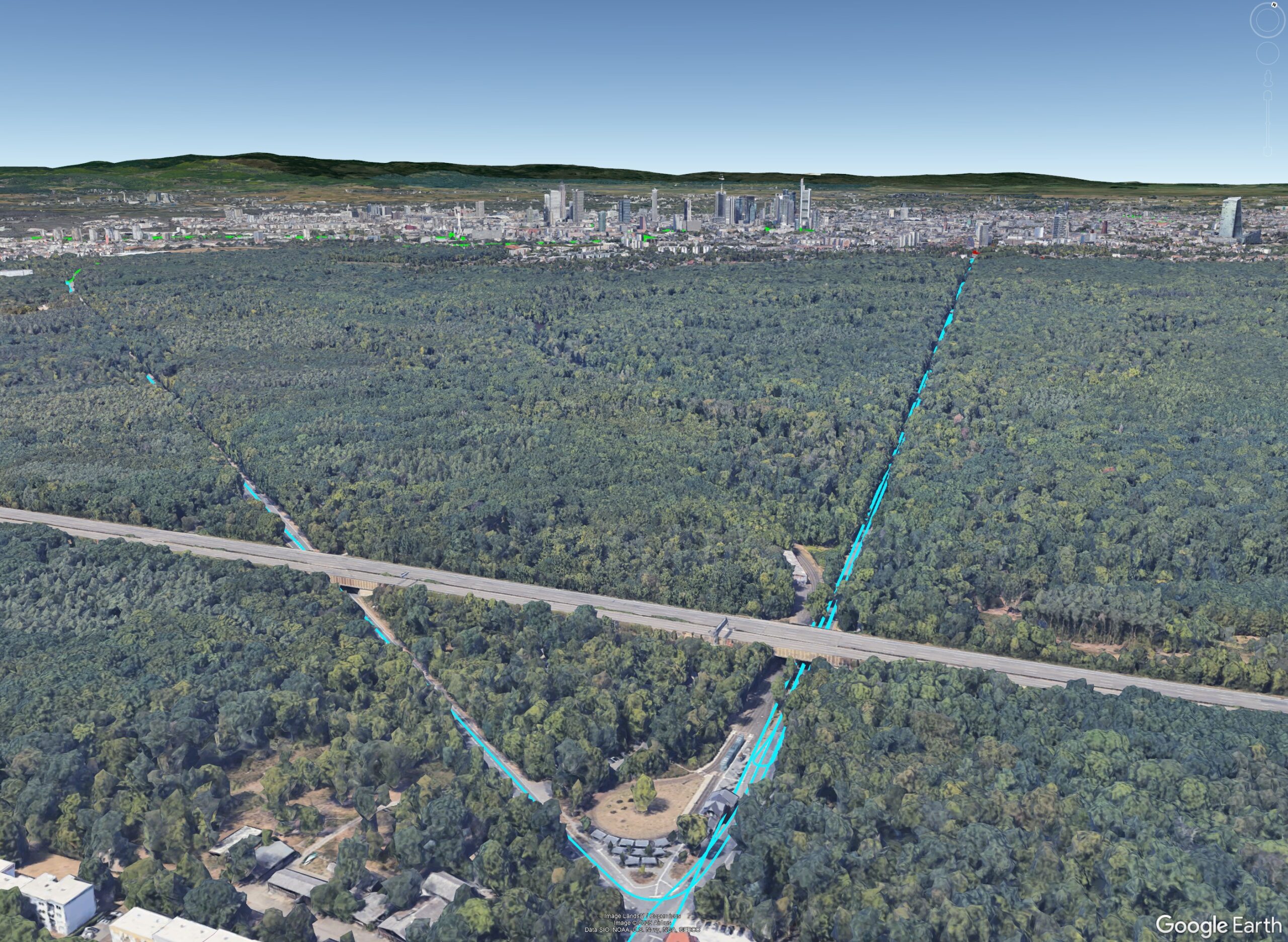
For this mini-series we use one consistent dataset: 20 drive logs, each close to one hour. We drove a normal passenger car in Darmstadt and Frankfurt through forest, city, dense residential, industrial zones, highway, and the high-rise/banking district. Hardware was a geodetic GNSS receiver (Javad Triumph-LS) and a MEMS IMU from ~2013 (Xsens MTi G-700). Processing uses AlgoNav’s tightly-coupled Network-PPK with our mobile VRS (MVRS), fused with IMU, odometry, and motion constraints. All five posts rely on these runs.

Forest is not “just a bit of attenuation”

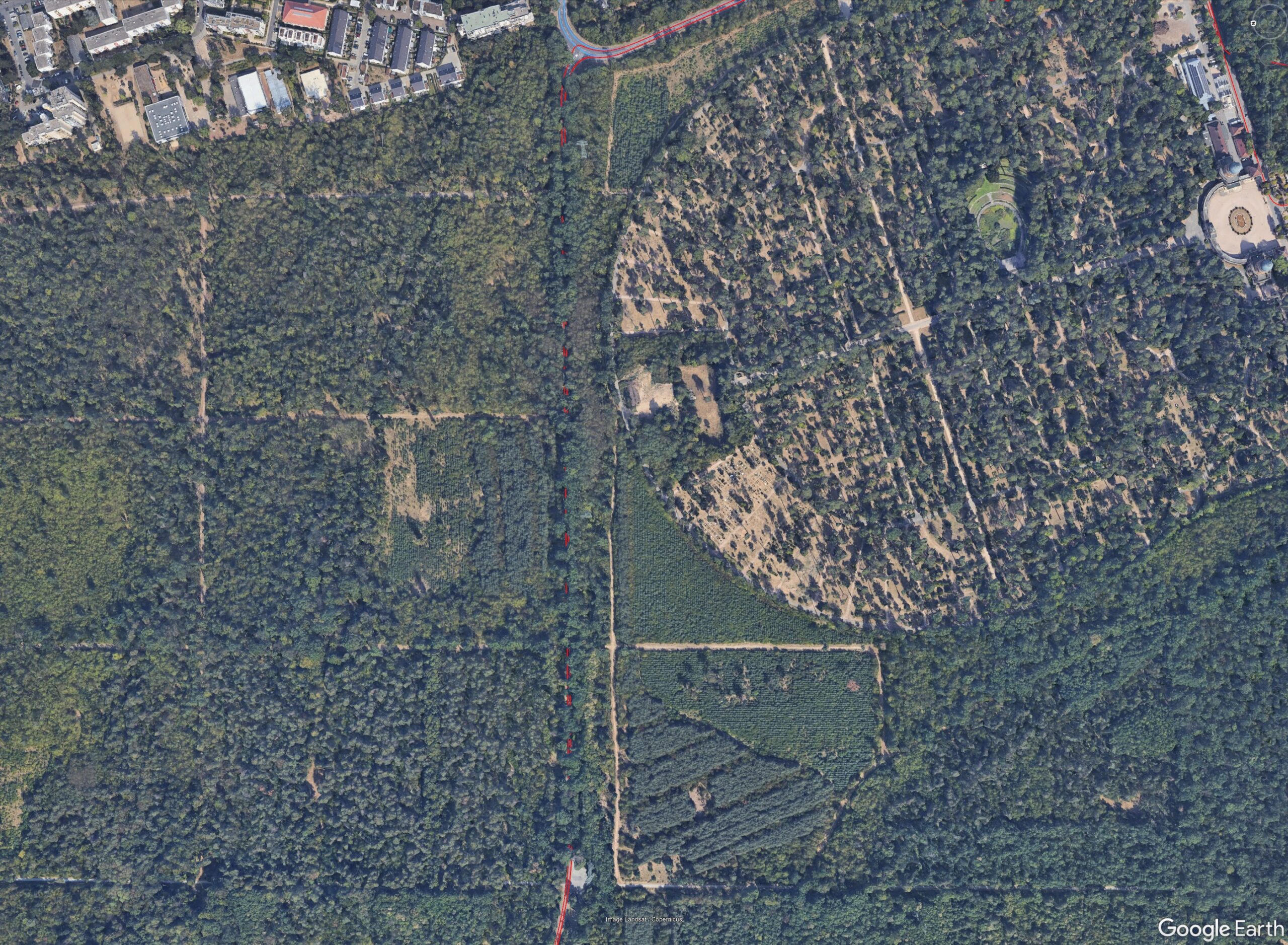
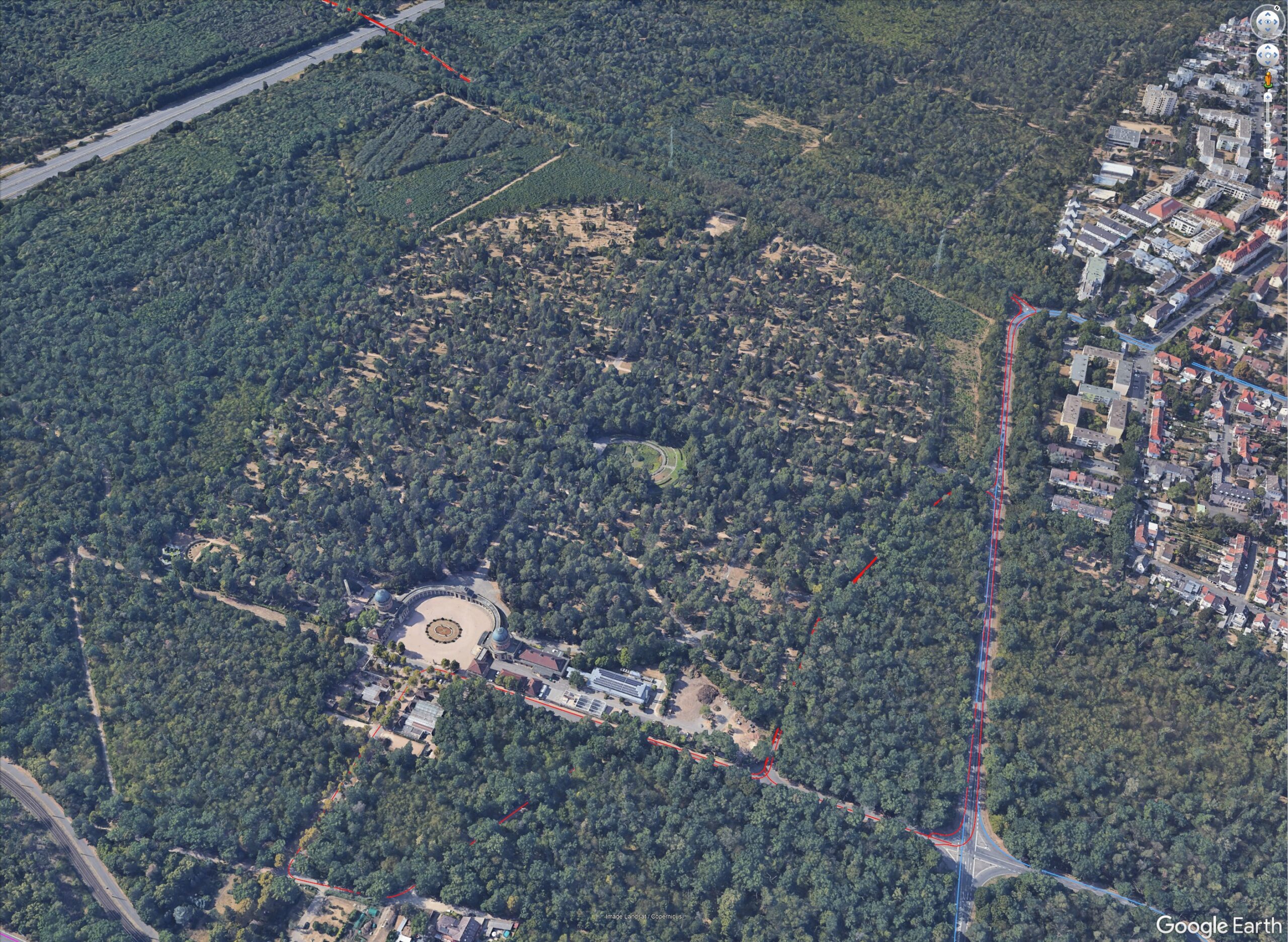
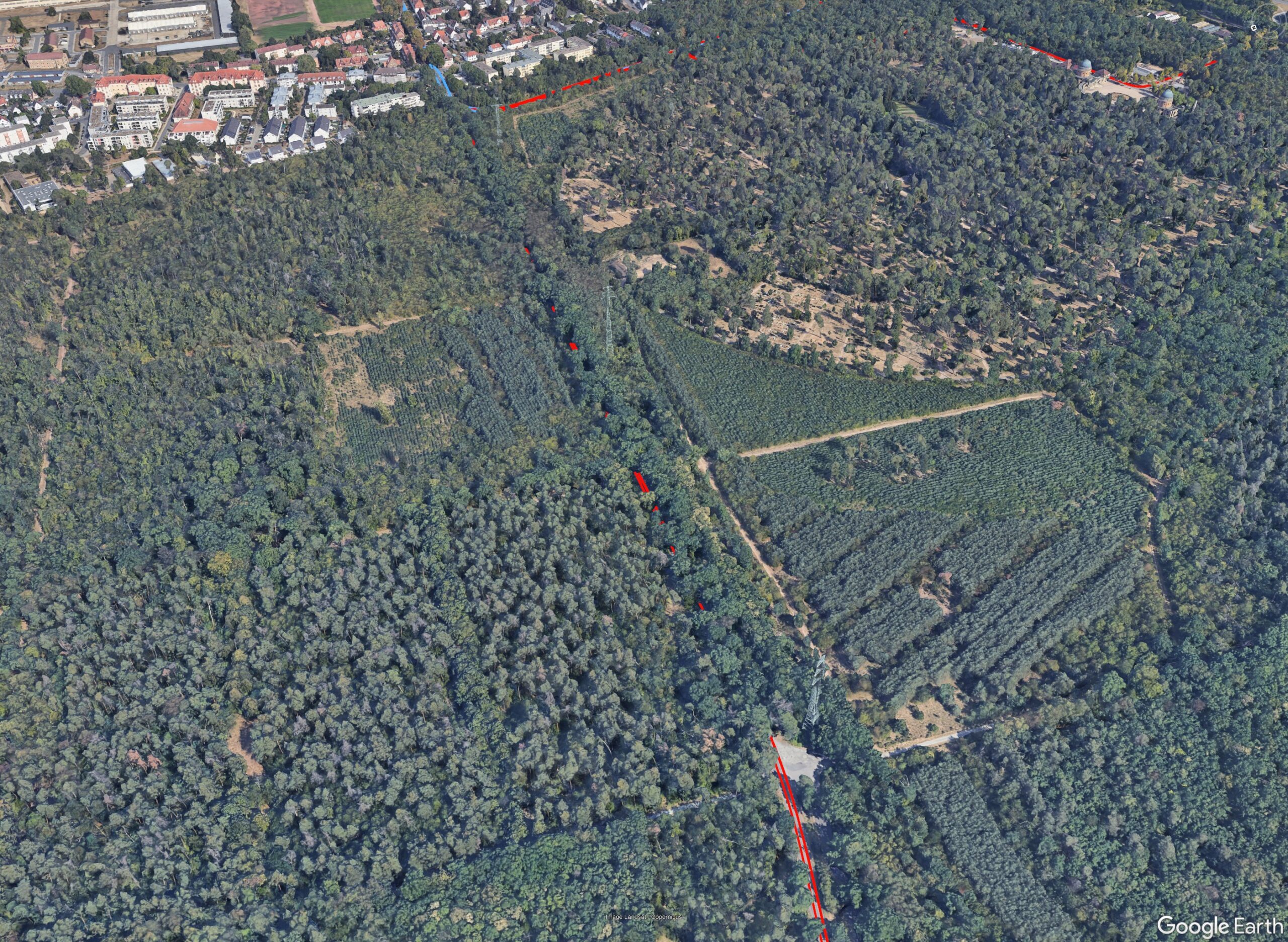
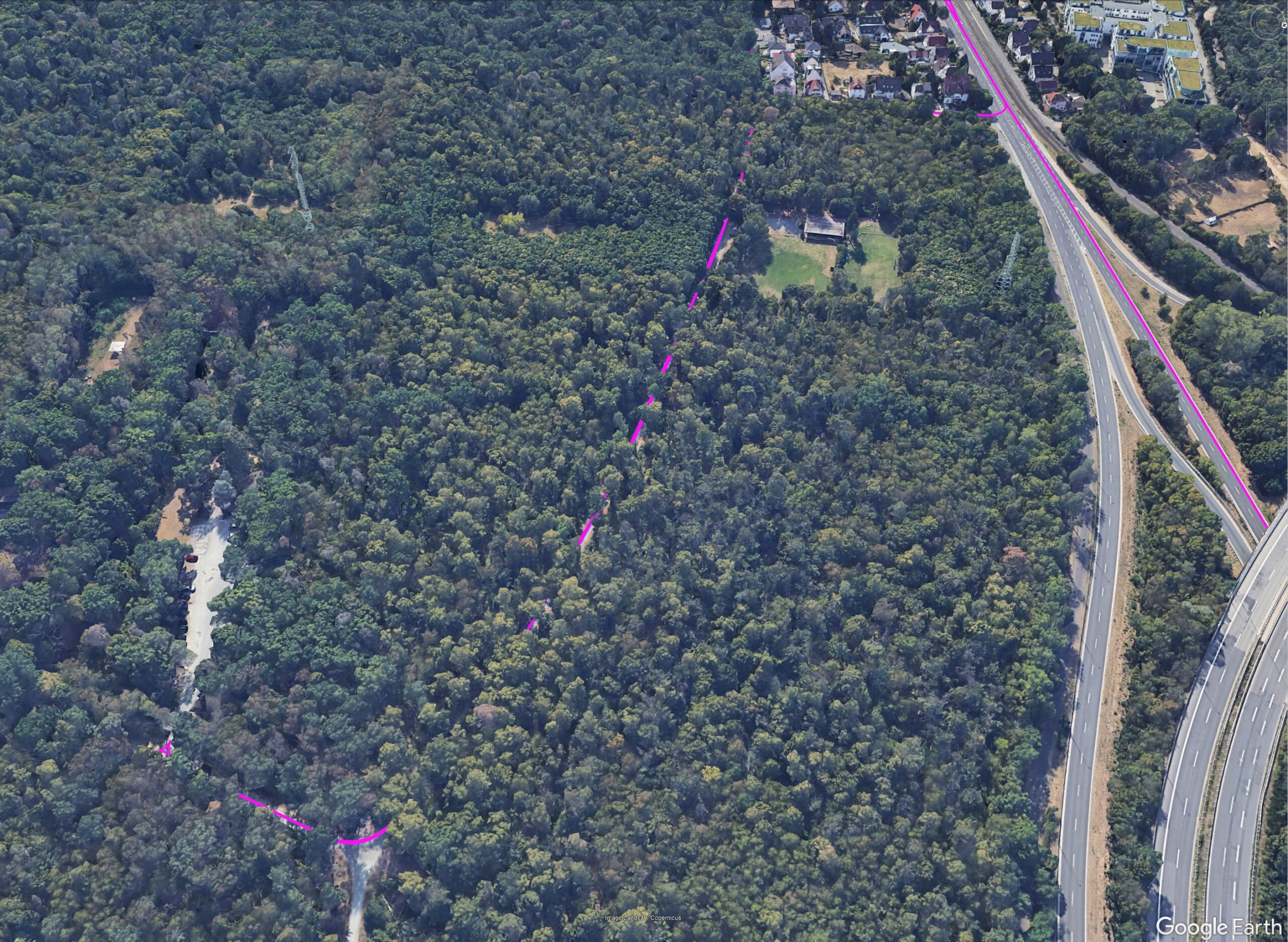
In dense forest the canopy is surprisingly hard on GNSS. Signals do not pass leaves and branches easily. When tree crowns even touch above the road, the receiver may see only a few satellites at any time.

There is one upside: vegetation has low reflectivity. So the signals we do receive are often cleaner (less multipath) than you might expect. The blocked ones are simply not tracked, or come with very low SNR, which a modern receiver marks as “unsafe”.

So, few satellites-but usable ones. Sounds manageable? Not the full story.

Geometry: many satellites, still poor position

On a road inside dense forest, the antenna often “sees” only the sky along the road corridor. Trees block the sides. The result: most visible satellites line up in roughly one direction (forward/backward) plus overhead.

You can even have 10 satellites and still be in a weak geometry: along-track (forward/backward) and vertical are fine, but lateral (cross-track) is poorly observed. In matrix terms: the design matrix tells the truth-your solution is close to singular in that lateral direction.

Standard estimators handle bad geometry in theory. They inflate covariance where information is weak. So are we safe? Not quite.

The trap: a single “helpful” side satellite

Sometimes a side satellite “blinks” through the canopy for a few seconds. In principle, this one satellite suddenly makes the lateral direction observable again. Great-if it is trustworthy.

The problem: with our forest geometry we have redundancy in along-track and vertical, but not in lateral. If that side satellite is biased (bad code/carrier, residual multipath from a trunk, half-blocked antenna pattern), there is no second sideways measurement to cross-check it. A classic outlier test may not detect the bias, because there is not enough independent information in that direction.

This is where Minimum Detectable Bias (MDB) comes in. MDB asks: Given my current geometry, what is the smallest bias that I could still detect reliably?

• If the MDB in lateral is large, a moderate bias on that single side satellite will sneak through undetected.
• If the MDB is small, we can detect even tiny biases confidently.

In dense forest, the lateral MDB is often large. So a reliability-first algorithm may down-weight or even ignore that single side satellite even when it looks fine by classic tests-simply because, if it were wrong, we could not detect it.

Yes, that means we trade some availability (fewer fixes using that satellite) for stronger reliability (no hard lateral jumps).

What a reliability-first filter does

A practical, conservative strategy in forest:

• Geometry-aware weighting: Increase measurement variance along the weak (lateral) direction. If only one side satellite supports lateral, treat it carefully.
• MDB-gated use: Use MDB thresholds to decide if a “just one” satellite can contribute to the solution or should be capped/ignored for safety.
• Time consistency with IMU/odometry: Tightly-coupled fusion keeps a smooth lateral estimate from the IMU when GNSS is weak. Short, clean side glimpses are integrated gradually, not as step changes.
• Selective fixing: Allow integer fixing when geometry supports it; otherwise hold float or partial constraints. The goal is to avoid “fixed-but-wrong” in lateral.
• Deferred optimism: If the side satellite proves stable over time (repeats, multiple short windows, consistent residuals), loosen the weight and let lateral accuracy improve.

This way, the reported covariance may be a bit pessimistic in lateral during canopy segments-but the trajectory stays trustworthy, with fewer irrecoverable slips.

What we see in our data

Typical forest segments show:

• 5–8 satellites visible, mostly aligned with the road; lateral dilution is high.
• SNR is either decent (clear lines of sight) or very low (blocked). Multipath is less chaotic than in urban glass, but still possible near trunks and wet leaves.
• Short side windows appear for 1–3 seconds at gaps in the canopy. With MDB-aware logic, we accept these windows only when they repeat or align with IMU prediction.
• The tightly-coupled filter keeps heading and along-track strong; lateral stays stable but conservative. When the canopy opens (small clearing, junction, bridge over the forest road), lateral tightens quickly.

Practical takeaways

• Few signals is okay; bad geometry is the real risk. Ten satellites in a line are worse than five with spread.
• Prefer reliability over aggressive fixes in lateral under canopy. A single “hero” satellite can do more harm than good.
• Use IMU and odometry to carry lateral knowledge across weak segments, then let GNSS re-tighten it when geometry improves.
• Watch MDB, not only residuals. If the MDB says you couldn’t detect a bias, treat that measurement with caution-even if it looks clean.
• Plan test routes with geometry in mind: include clearings, crossings, or short elevated segments to re-condition lateral.

What this means for your projects

If your vehicles run in forests or tree-lined rural roads, expect stable along-track and vertical, but fragile lateral during dense canopy. A reliability-first approach-MDB-aware weighting, tightly-coupled GNSS/IMU, and careful acceptance of side glimpses-keeps maps and trajectories usable without hidden surprises.

This was Part 2 of our five-post series on tough GNSS environments:

1. Underpasses
2. Forest (this post)
3. “European Urban Canyon” (very narrow, low-rise residential streets)
4. Tunnels and dense tunnel exits
5. Urban Canyon (the classic high-rise case)

If you have forest segments to share, we’re happy to compare geometry stats and MDB patterns. Next up: the European Urban Canyon-why two-to-three-story streets can behave like a miniature skyline.