GNSS/IMU-Positioning Urban Challenges #1: Underpasses

Short intro and dataset
For this mini-series we use one consistent dataset: 20 drive logs, each close to one hour. We drove a normal passenger car through many scenes in Darmstadt and Frankfurt: forest, city, dense residential, industrial zones, highway, and also high-rise/banking district. The setup was a geodetic GNSS receiver (Javad Triumph-LS) and a MEMS IMU from ~2013 (Xsens MTi G-700). Processing is done with AlgoNav’s tightly-coupled Network-PPK using our mobile VRS (MVRS) plus fusion with IMU, odometry, and motion constraints. All five posts in this series are based on these same runs.

Part 1 – “Typical” underpasses (driving under bridges)

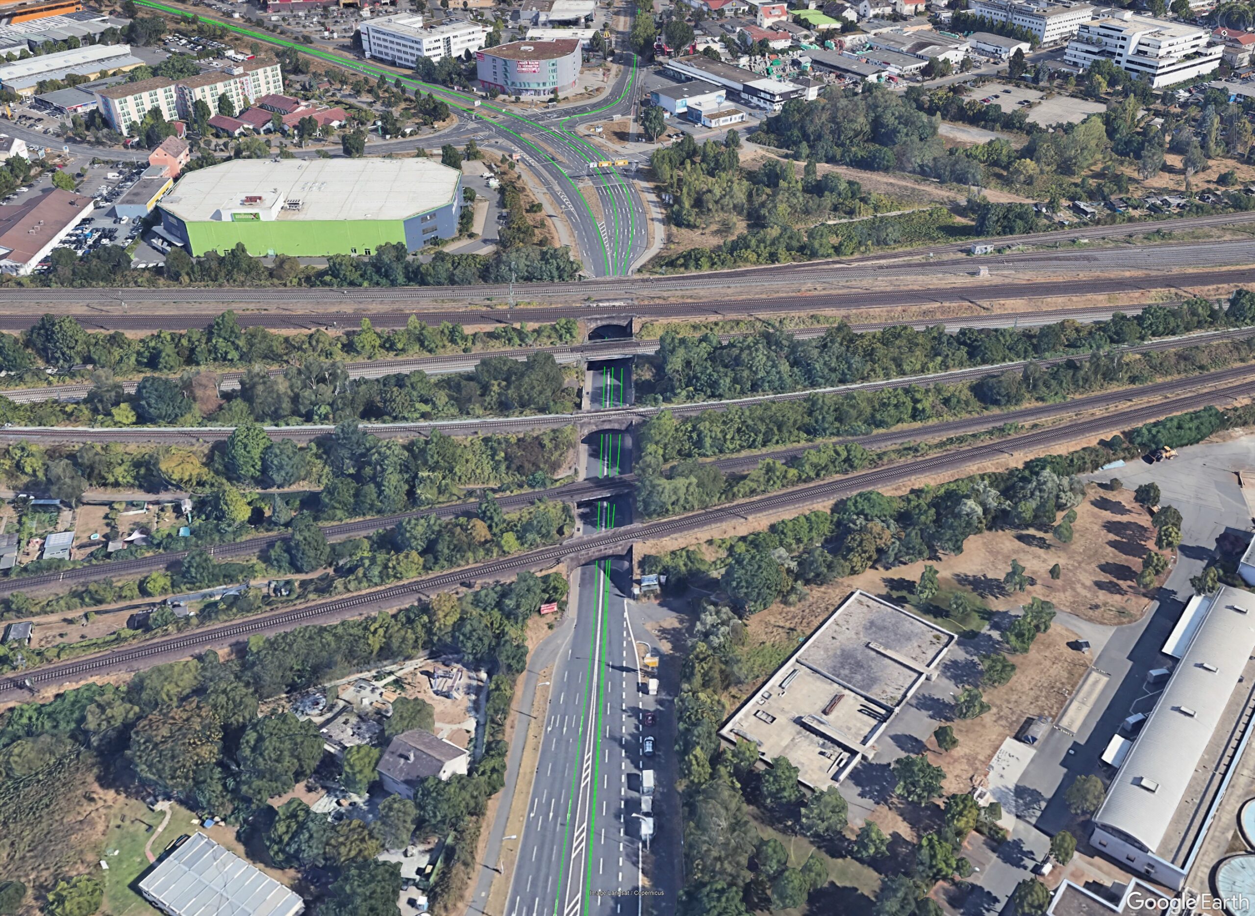
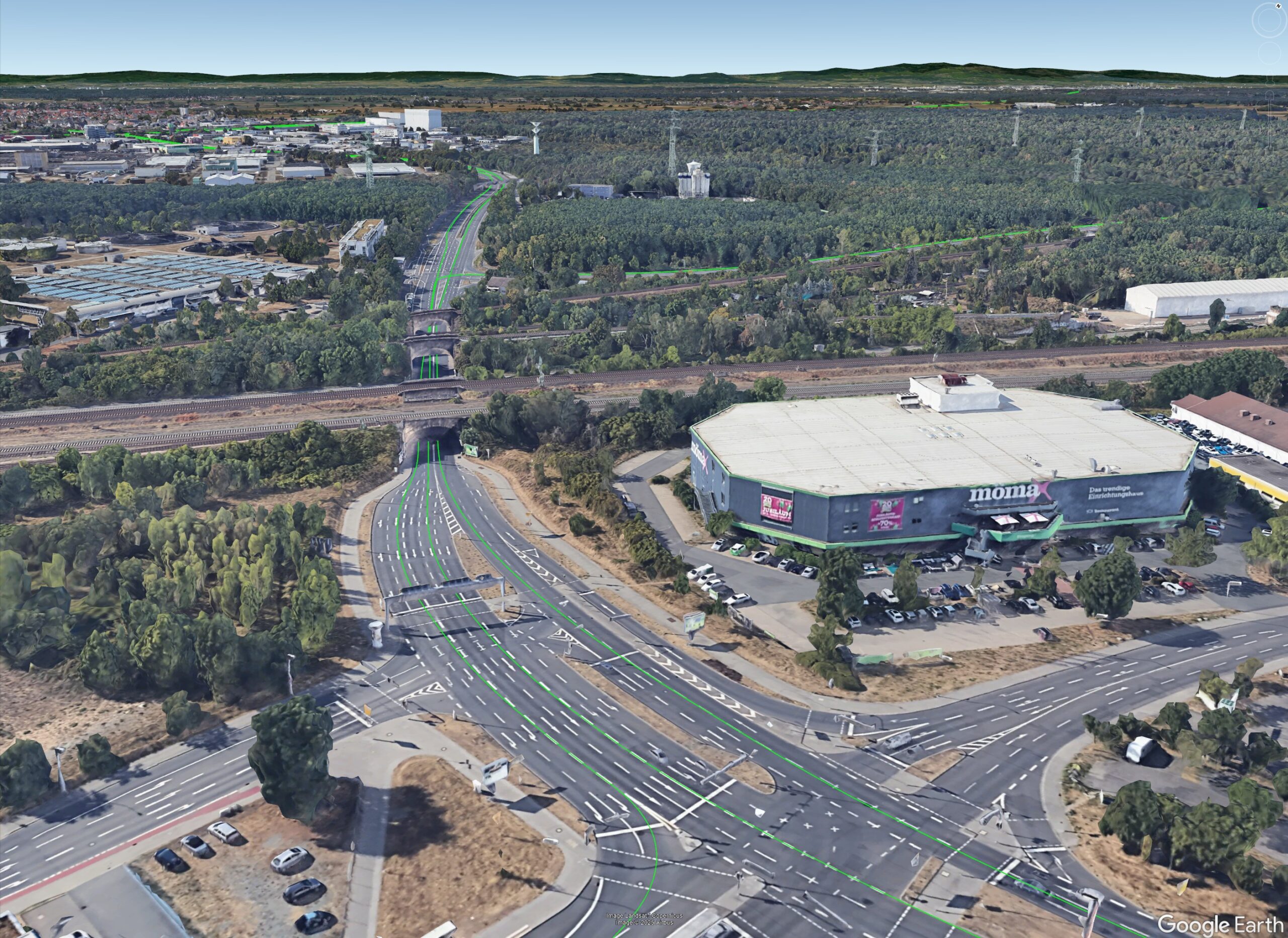
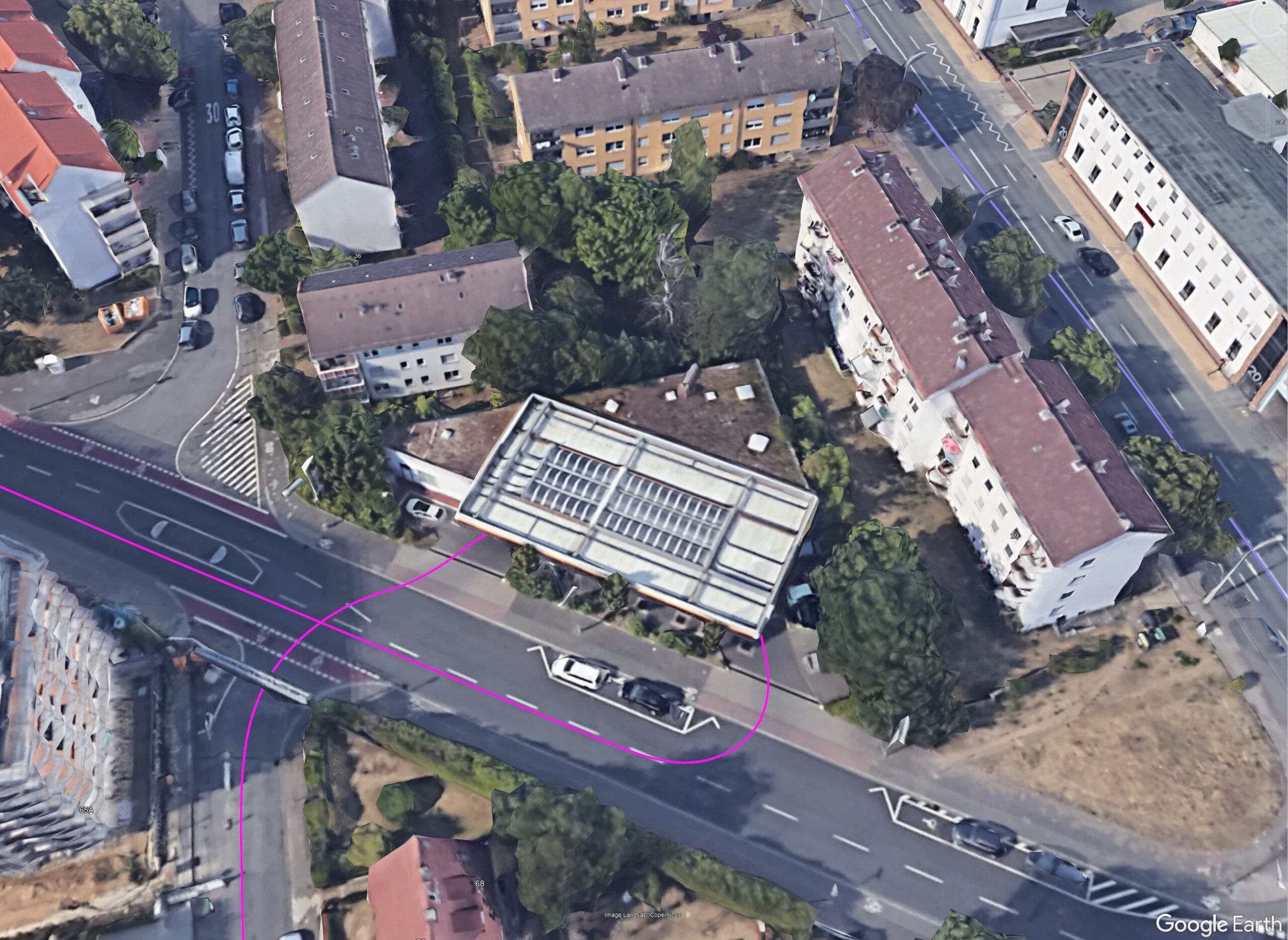
Short underpasses are not the dramatic enemy they look like. The IMU can bridge short outages quite well. Still, there are two important things to keep in mind for high-accuracy positioning.

1) Real-time fix needs to re-lock after a full break.
In many real-time systems, a carrier-phase ambiguity fix will drop when all satellites are lost, even for one second. After the bridge, the engine must fix again. This re-fix costs time and meters, and it can repeat if you drive through several underpasses in quick sequence. The result is a “staircase” of small errors.

2) Post-processing gives us time symmetry.
In post-processing we are not forced to go only forward in time. We can also solve ambiguities backwards. That means we approach the bridge from both directions in time and stabilize the ambiguities from “before” and “after”. This reduces the unfixed gap and often turns it into a fully fixed stretch.

Why tightly-coupled GNSS/IMU matters here
A tightly-coupled filter feeds raw GNSS (including carrier phases) and IMU together. Even if GNSS is temporarily blind, the filter keeps a very good IMU-predicted position and velocity. When the first satellites show up again-sometimes only two or three, and sometimes only for 1–3 seconds-that prediction shrinks the search space for integer fixing. Practically, this means:

• You often get a re-fix at the very first re-acquisition, not several seconds later.
• In sequences of multiple short underpasses, you can stay in fixed most of the time, or at least re-fix faster between them.
• The overall trajectory stays tighter, especially heading and cross-track position.

Typical scene we see in the data

• Enter underpass → complete GNSS break for ~1–2 s.
• IMU holds pose; odometry/motion constraints prevent unrealistic drift.
• Exit underpass → 2–3 satellites visible briefly → ambiguities re-fixed immediately.
• Next bridge 5 seconds later → same story, still stable.

This is not magic; multipath and bad geometry still exist. But with a good tightly-coupled solution and bi-directional ambiguity fixing in post-processing, these short gaps stop being a big problem.

Part 2 – Pivot satellite in double differences: why “dynamic” wins

If you do double-differenced carrier-phase (classic PPK/RTK), you always have a pivot (reference) satellite. Many systems simply choose “the highest elevation satellite is the pivot”. That rule is simple-but under bridges it is also fragile.

What goes wrong with a rigid pivot
Under a narrow bridge, the set of visible satellites shifts fast. On entry, satellites behind you are more visible; on exit, satellites ahead of you come first. If your pivot is fixed to “highest” and that satellite gets blocked for a moment, your whole double-difference network is stressed. You can lose fix, even though several other satellites were still fine.

AlgoNav’s approach: dynamic pivot satellite switching
We switch the pivot on the fly, based on quality metrics (visibility, SNR, tracking flags, geometry). The switch is safe for the integer state, so we do not throw away the fixed solution just because the pivot changed. In effect:

• Under very narrow bridges, we keep integer fix continuously, because the pivot follows the visibility window.
• In rapid visibility transitions (rear-visible on entry, front-visible on exit), the pivot switches accordingly-no hard reset needed.
• During short stops under roofs (e.g., gas station canopy), the “highest satellite wins” rule completely fails: the highest one might be blocked by the roof beam. With dynamic pivoting we can even use a low-elevation but stable satellite as pivot. That keeps a fixed solution while you are stationary.

Bonus under a canopy: better IMU bias estimation
When your car stands still for a minute under a gas station roof, a stable fixed solution is gold. The filter can observe IMU biases in a quiet condition (no vehicle dynamics), which later improves the whole run. With a rigid pivot strategy, the solution would drop to float or dead-reckoning, and those bias estimates would be worse.

Practical takeaways

• Short GNSS blackouts are normal under bridges. With a tightly-coupled filter, the IMU covers those seconds without big drift.
• Post-processing reuses time in both directions, so ambiguity fixing can “meet in the middle” at the bridge.
• Dynamic pivot switching keeps the double-difference network stable when visibility changes fast.
• Under canopies, a flexible pivot (even at low elevation) can maintain a fixed solution and helps estimate IMU biases while stationary.

What this means for your projects

If your vehicles operate in European cities, you know the pattern: small bridges, rail overpasses, repetitive shading between buildings, short stops under roofs. The combination of tightly-coupled Network-PPK + dynamic pivot switching + bi-directional fixing is designed exactly for that. It does not remove physics, but it changes how often you stay fixed and how fast you recover-often the difference between a “usable” lane-level map and one with holes.

This was Part 1 of our five-post mini-series on the hardest GNSS environments we see in real roads:

1. Underpasses (this post)
2. Forest
3. “European Urban Canyon” (very narrow, low-rise residential streets)
4. Tunnels and dense tunnel exits
5. Urban Canyon (the “classic” high-rise case)

If you want to compare notes or share your own tricky segments, we’re happy to exchange data and methods. In the next post we move to Forest-low elevation satellites, canopy attenuation, and what selective fixing can do there.